Graphs
- Representation
- Adjacency Matrix
- Adjacency Lists
- Traversal schemes
- DFS (Depth First Search)
- Breadth First Search (BFS)
- Minimal Spanning
- Kruskal
- Prim
Graph: A graph consists of a set of nodes (vertices) and a set of arcs (or edges).
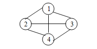
- The set of nodes {1,2,3,4}
- The set of arcs or edges {(1,2), (1,3), (1,4), (2,4), (2,3), (3,4)}
Thus a graph G consists of two sets V and E. V is a finite non-empty set of vertices. E is a set of pairs of vertices. These pairs are called edges. V(G) and E(G) will represent the sets of vertices and edges of graph G.
Thus, we may write G=(V,E) to represent a graph.
| Tree | Graph |
| Root | No root |
| Parent-child relationship | No such relationship |
| Connected | May be disconnected |
| acyclic | May contain cycle |
| (do not contain any cycle) |
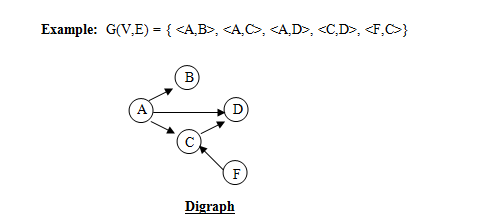
Directed Graphs: If the pairs of nodes/vertices that make up the arcs are ordered pairs (direction of movement is used) the graph is said to be a directed graph (or digraph).
NOTE:
- The arrows between nodes represent arcs. The head of each arrow represents the second ndoe in the ordered pair of nodes making up an arc, and the tail of each arrow represents the first node in the pair.
- We use parenthesis to indicate an unordered pair and angular brackets to indicate an ordered pair.
- A graph need not be a tree but a tree must be a graph.
- Nodes need not have any arc associated with them.
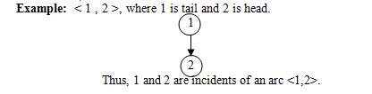
Incident Node: A node n is incident to an arc x, if n is one of the two nodes in the ordered pair of nodes that constitute x. (We may also say that x is incident to n).
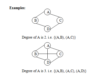
Degree of a node: The degree of a node is the number of arcs incident to it.
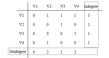
Indegree: The indegree of a node n is the number of arcs that have n as the head. (Arrows coming in n).
Example:
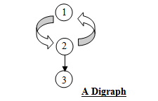
Outdegree: The outdegree of n is the number of arcs that have n as the tail. In the above graph, outdegree of 3 is 0 as it has no other node, for which it is a tail.
Outdegree of 2 is 2 i.e. {<2,1>, <2,3>}
Note: Maximum number of edges in any n vertex undirected graph is n(n-1)/2
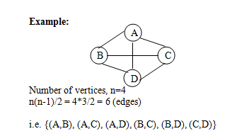
Complete Graph: A n vertex undirected graph with exactly n(n-1)/2 edges is said to be a complete graph.
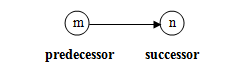
Adjacent node: A node n is adjacent to a node m if there is an arc from m to n. If n is adjacent to m, n is called a successor of m and m is called a predecessor of n.
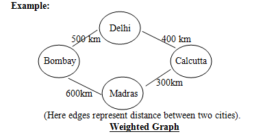
Weighted Graph or Network: When a number is associated with each arc/edge i.e. edges have properties or attributes the graph is called a weighted graph or a network.
- Adjacency Matrix
- Adjacency Lists
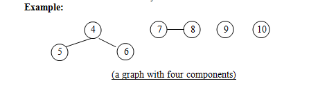
Connected Graph: A graph is said to be connected if every pair of vertices in a graph is connected.
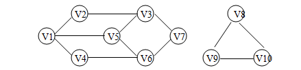
Component of a graph: A component of a graph is a maximal connected subgraph. In the above example there are two components.
(i) Adjacency Matrix Representation: A graph g with n vertices can be represented by a n*n matrix.

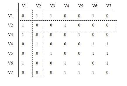
Since the above graph has 7 vertices, hence it can be represented by 7 X 7 matrix.
Computing Degree of a Vertex:
(i) For an undirected graph:- Degree is equal to sum of corresponding row = sum of corresponding column. For example: In the above table Degree of V2 = sum of row corresponding to V2 = sum of column corresponding to V2. (as shown by dotted lines), which is 2.
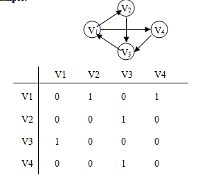
(ii) For a directed graph:-
Number of vertices = 4
Order of Adjacency Matrix = R x C = 4 x 4
Note:
- Sum of 1’s of the row gives outdegree.
- Sum of 1’s of the columns gives indegree.
- Sum of indegree + outdegree gives degree of that node
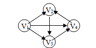
Example: In the above figure, Outdegree of V1 is 3 and Indegree of V1 is 0. Thus, Degree of V1 is 3+0=3.
Adjacency Matrix for the above digraph is given below:
Finding total number of nodes:
(i) For an undirected graph: To find the total number of edges of the graph, we find the sum of all 1’s except diagonal and divide it by 2 and add all 1’s of the diagonal.
Example:
Total number of edges = Sum of all 1’s except diagonal
= 8/2 = 4 + all 1’s of the diagonal ([ ]), which are all zero.
Thus, total number of edges = 4
(ii) For a directed graph: For a directed graph, total number of edges are given by sum of all 1’s.
Example:
Total number of edges = 5
Implementation of Adjacency Matrix:
Example 1:
Program to implement the above graph is as follows:
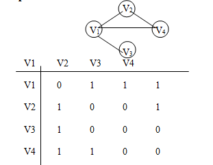
Adjacency List: We have an array of n elements (for a graph of n vertices). Each element has a linked list associated with it, which corresponds to the vertices, which are adjacent to the vertex.
NOTE:
- Adjacent of node V1 is V2 and V3.
- Adjacent of node V2 is V1 and V4.
- Adjacent of node V3 is V1 and V4.
- Adjacent of node V4 is V2 and V3.
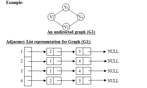
For Graph G1:
- Total number of edges in the graph = (Total number of nodes)/2 = 8/2 = 4 edges.
- Degree of a vertex can be found by counting the number of nodes for that particular value.
- Degree of vertex V1 = 2
- Degree of vertex V2 = 2
- Degree of vertex V3 = 2
- Degree of vertex V4 = 2
For a directed graph:
- Total number of edges in graph is equal to total number of nodes.
- Degree of a node is equal to number of nodes for that vertex.
- Outdegree of a vertex can be found out by simply counting the nodes of that element.
The indegree is calculated by traversing all the nodes and counting the occurrences of that vertex.
NOTE:
- Adjacent of node V1 is V2, V3 and V4.
- Adjacent of node V2 is V3, V4 and V5.
- Adjacent of node V3 is V5.
- Adjacent of node V4 is V5.
- Adjacent of node V5 is V4.
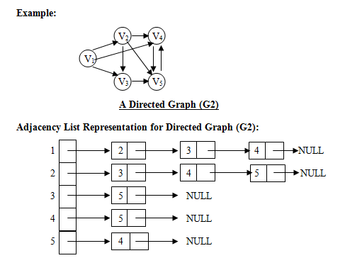
For Graph G2:
- Total number of edges = Total number of nodes = 9
- Degree of a node = Number of nodes for that vertex
- Degree of V1 = 3
- Degree of V2 = 3
- Degree of V3 = 1
- Degree of V4 = 1
- Degree of V5 = 1
– Outdegree of a vertex = Number of nodes of that vertex.
- Outdegree of V1 is 3
- Outdegree of V2 is 3
- Outdegree of V3 is 1
- Outdegree of V4 is 1
- Outdegree of V5 is 1
– Indegree of a vertex = Traverse all nodes and count the occurrences of that vertex.
- Indegree of V1 = The occurrence of V1 is 0 (zero) i.e. no occurrence. Hence its indegree is zero.
- Indegree of V2 = 1 (since out of 9 nodes, it is visible only once).
- Indegree of V3 = 2
- Indegree of V4 = 3
- Indegree of V5 = 3
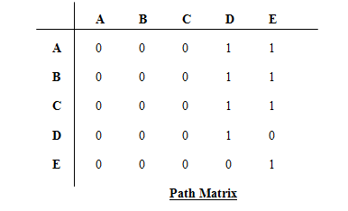
adj[i][k] and adj[k][j] are TRUE.
which means that there is an arc from i to node k and an arc from k to node j. Thus adj[i][k] && adj[k][j] equals TRUE if an only if there is a path of length 2 from i to j passing through k.

Consider an array adj2 such that adj2[i][j] is the value of the foregoing expression. adj2 is called the path matrix of length 2. adj[i][j] indicates whether or not there is a path of length 2 between i and j. Consider the following example:
The Adjacency Matrix for the above graph is shown below:
The path matrix for the above adjacency matrix is as follows:
Traversal schemes:
- DFS (Depth First Search)
- BFS (Breadth First Search)
DFS (Depth First Search): We move depth-wise i.e. we start from the first node (any of the vertex) and then visit the node that is adjacent to it. Then from that node we move to the vertex adjacent to it and so on. If we can’t move further, then return to the previous node and continue. We keep on marking the nodes which we have already visited.
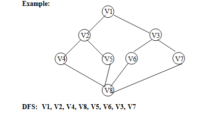
BFS (Breadth First Search): After a node is visited, we first visit all the vertices adjacent to it.
Example: Refer to the above graph. BFS traversal result is-
V1, V2, V3, V4, V5, V6, V7, V8
Spanning trees: Spanning trees have two basic properties-
(i) acyclic
(ii) connected
If we define a subgraph of this graph, then all such possibilities that define it as a subgraph with no cycle may be referred to as spanning tree.
If the graph is a weighted graph, then it is often desired to create a spanning tree T for G such that the sum of weights of the tree edges in T is as small as possible. Such a tree is called a minimum spanning tree and represents the cheapest way of connecting all the nodes in G.
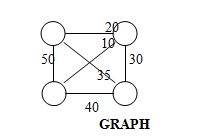

The dotted subgraph with least weight 60 is an example of minimum cost spanning tree, as it has minimum weight value.
There are a number of techniques for creating a minimum spanning tree for a weighted graph:
- Prim’s Algorithm
- Kruskal’s algorithm
- Round Robin Algorithm
An arbitrary node is chosen initially as the tree root. The nodes of the graph are then appended to the tree one at a time until all nodes of the graph are included.
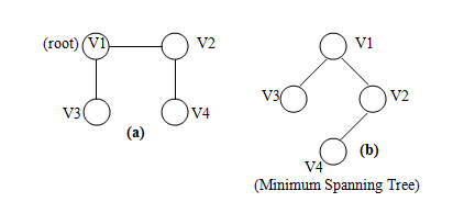
In figure (a), V1 is taken to be root of the tree, which is an arbitrary node chosen as a root. Adjacent of V1 is V2 and V3. V2 becomes the right child of V1 and V3 becomes the left child of V1 in the tree as shown in fig (b).
The nodes of the graph are initially considered as n distinct partial trees with one node each. At each step of the algorithm two distinct partial trees are connected into a single partial tree by an edge of the graph. When only one partial tree exists, it is a minimum spanning tree.
The issue is what connecting arc to use at each step. The answer is to use the arc of minimum cost that connects two distinct trees. To do this, the arcs can be placed in a priority queue based on weight. The arc of lowest weight is then examined to see if it connects two distinct trees.
An ascending order priority queue is constructed that contains the weights of the arcs of the given graphs as shown in the following figure:
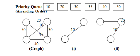
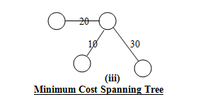
Any further insertion is not required since number of vertices is equal to 4, which is the same as the total number of vertices in the given graph. Thus lower weights are chosen to construct minimum spanning tree.
3. Round Robin Algorithm (given by Tarjan & Cheriton):
It is similar to Kruskal’s algorithm except that there is a priority queue of arcs associated with each partial tree rather than one global priority queue of all un-examined arcs.
All partial trees are maintained in the queue, Q. Associated with each partial tree T, is a priority queue. P(T) of all arcs with exactly one incident node is the tree ordered by the weights of the arcs.